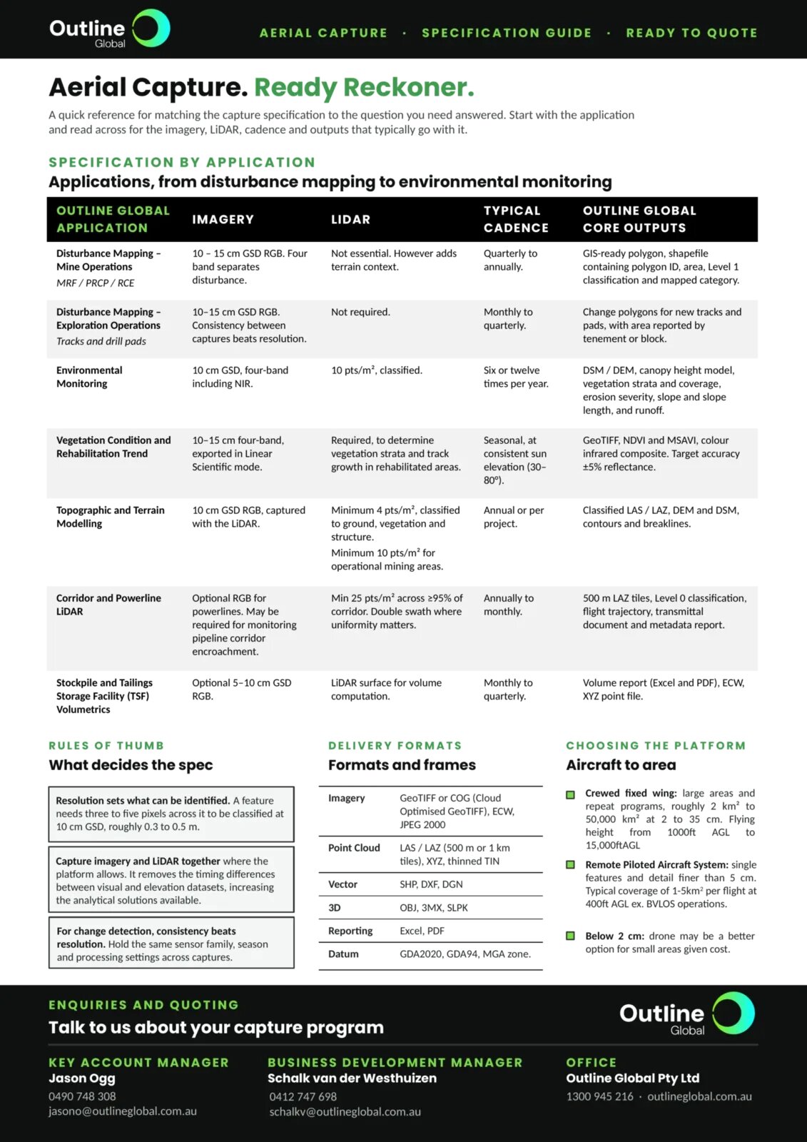

A quick reference for matching the capture specification to the question you need answered. Start with the application and read across for the imagery, LiDAR, cadence and outputs that typically go with it. The same guide is available as a one-page image at the end of this article.
Specification by application
Applications, from disturbance mapping to environmental monitoring.
| Application | Imagery | LiDAR | Typical cadence | Core outputs |
|---|---|---|---|---|
| Disturbance mapping, mine operations (MRF / PRCP / RCE) | 10 to 15 cm GSD RGB. Four band separates disturbance. | Not essential. However adds terrain context. | Quarterly to annually. | GIS-ready polygon, shapefile containing polygon ID, area, Level 1 classification and mapped category. |
| Disturbance mapping, exploration operations (tracks and drill pads) | 10 to 15 cm GSD RGB. Consistency between captures beats resolution. | Not required. | Monthly to quarterly. | Change polygons for new tracks and pads, with area reported by tenement or block. |
| Environmental monitoring | 10 cm GSD, four-band including NIR. | 10 pts/m², classified. | Six or twelve times per year. | DSM / DEM, canopy height model, vegetation strata and coverage, erosion severity, slope and slope length, and runoff. |
| Vegetation condition and rehabilitation trend | 10 to 15 cm four-band, exported in Linear Scientific mode. | Required, to determine vegetation strata and track growth in rehabilitated areas. | Seasonal, at consistent sun elevation (30 to 80°). | GeoTIFF, NDVI and MSAVI, colour infrared composite. Target accuracy ±5% reflectance. |
| Topographic and terrain modelling | 10 cm GSD RGB, captured with the LiDAR. | Minimum 4 pts/m², classified to ground, vegetation and structure. Minimum 10 pts/m² for operational mining areas. | Annual or per project. | Classified LAS / LAZ, DEM and DSM, contours and breaklines. |
| Corridor and powerline LiDAR | Optional RGB for powerlines. May be required for monitoring pipeline corridor encroachment. | Min 25 pts/m² across ≥95% of corridor. Double swath where uniformity matters. | Annually to monthly. | 500 m LAZ tiles, Level 0 classification, flight trajectory, transmittal document and metadata report. |
| Stockpile and Tailings Storage Facility (TSF) volumetrics | Optional 5 to 10 cm GSD RGB. | LiDAR surface for volume computation. | Monthly to quarterly. | Volume report (Excel and PDF), ECW, XYZ point file. |
Rules of thumb: what decides the spec
- Resolution sets what can be identified. A feature needs three to five pixels across it to be classified at 10 cm GSD, roughly 0.3 to 0.5 m.
- Capture imagery and LiDAR together where the platform allows. It removes the timing differences between visual and elevation datasets, increasing the analytical solutions available.
- For change detection, consistency beats resolution. Hold the same sensor family, season and processing settings across captures.
Delivery formats: formats and frames
| Product | Formats |
|---|---|
| Imagery | GeoTIFF or COG (Cloud Optimised GeoTIFF), ECW, JPEG 2000 |
| Point cloud | LAS / LAZ (500 m or 1 km tiles), XYZ, thinned TIN |
| Vector | SHP, DXF, DGN |
| 3D | OBJ, 3MX, SLPK |
| Reporting | Excel, PDF |
| Datum | GDA2020, GDA94, MGA zone |
Choosing the platform: aircraft to area
- Crewed fixed wing: large areas and repeat programs, roughly 2 km² to 50,000 km² at 2 to 35 cm. Flying height from 1,000 ft AGL to 15,000 ft AGL.
- Remote Piloted Aircraft System: single features and detail finer than 5 cm. Typical coverage of 1 to 5 km² per flight at 400 ft AGL, excluding BVLOS operations.
- Below 2 cm: a drone may be a better option for small areas given cost.
Enquiries and quoting
Talk to us about your capture program.
- Key Account Manager: Jason Ogg, 0490 748 308, jasono@outlineglobal.com.au
- Business Development Manager: Schalk van der Westhuizen, 0412 747 698, schalkv@outlineglobal.com.au
- Office: Outline Global Pty Ltd, 1300 945 216, outlineglobal.com.au